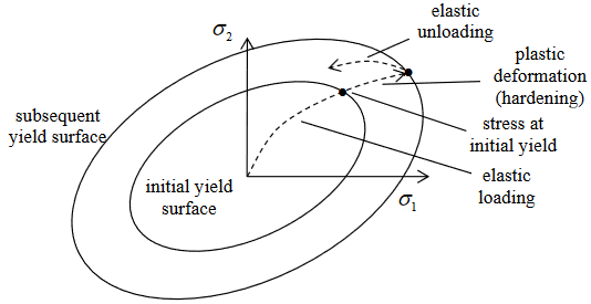
The hardening law, also known as hardening rules, describes how the yield surface changes under the plastic deformation. The hardening rule governs the change in material strength as the plastic material deformation. The change in material strength can also be thought of as a change in the geometry or position of the yielding surface. The developed yield surface is often called as the loading surface.
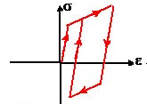
In the perfectly plastic case, plastic deformation starts to happen when the stress reaches the yield A point during the stress is maintained there. When the stress is reduced, elastic unloading occurs. In the hardening law, once yield occurs, the stress needs to keep increasing for forming of plastic deformation. If the stress is constantly held at B, no further plastic deformation will be occurred.
Strain Hardening Laws
Strain hardening, also known as work hardening, is the strengthening of a metal or polymer by plastic deformation. This strengthening occurs because of dislocation movements and generation within the crystal structure of the material.
Strain Hardening is when a metal is strained beyond the yield point. An increasing stress is required to produce additional plastic deformation, then the material becomes stronger and more difficult to deform. The resistance of the material to plastic flow will be increased that is called “Strain Hardening”.
The mixed hardening law is used when the loading surface may follow a combination of isotropic and kinematic hardening rules to capture both loading surface expansion and translation.
In this article, isotropic and kinematic hardening rules will be mentioned.
Isotropic Hardening
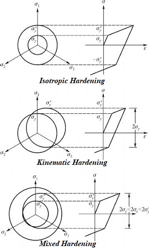
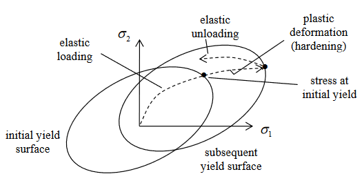
The isotropic hardening is simplest way to model a strain hardening, and it set the yield surface increase in size, but remain the same shape as a result of plastic straining, which means the yield surface remains uniform (without any distortion or translation), but expands with increasing stress.
The yield surface expands uniformly in all directions with plastic flow. The value of isotropic hardening is directly related to the amount of strain.
Isotropic hardening is related to the accumulated dislocation structure and expands the yield surface of a material under plastic deformation.

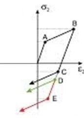
Plastic flow begins at the A point. The material yielding and plastic deformation will continue along its original stress strain path if the material is unloaded from the B point to zero stress and then reloaded.
As loading continues to the C point, isotropic hardening considers as the new yield strength of the material. Yielding will not occur until at the D point if the material is loaded in compression. The yield surface expands equally in all directions during plastic deformation with no distortion in shape and no translation of the yield surface centre.
The shape of the yield function is specified by the initial yield function and its size changes as the hardening parameter changes.
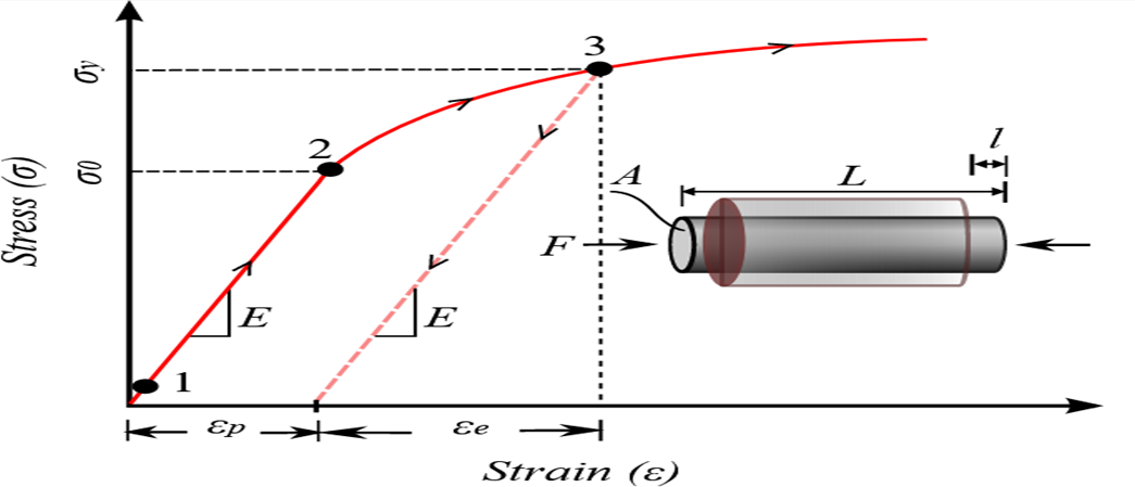
The effective plastic strain, which controls the hardening, can be defined using two different methodologies.
First, ɛp can be defined as the accumulated plastic strain according to the uniaxial state of stress.
Second, ɛp can be described using the plastic work per unit volume where σe is the effective stress defined based on the loading surface.
Different relations can be considered between the hardening parameter and effective plastic strain ɛp. For example, in the case of von Mises loading surface, the linear isotropic hardening can be selected as the simplest relation
In cyclic loading, an isotropic hardening model provides a poor representation of the stress-strain response for many metals. Also, isotropic hardening law is not useful in situations where components are subjected to cyclic loading. It does not account for Bauschinger effect and so predicts that after a few cycles the solid will just harden until it responds elastically.
The yield function formula:
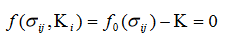
Isotropic hardening can then be expressed as:
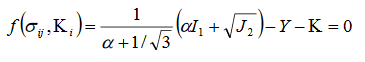
Y: The yield stress
K : Hardening parameter
Kinematic Hardening
In kinematic hardening, the yield surface is allowed to translate in stress space with no change in size or shape which means the yield surface remains the same shape and size but translates in the direction of yielding.
An initially isotropic plastic behaviour is no longer isotropic after yielding (kinematic hardening is a form of anisotropic hardening).
Kinematic hardening is one of the hardening rules describes the behavior of material after reaching yield surface.
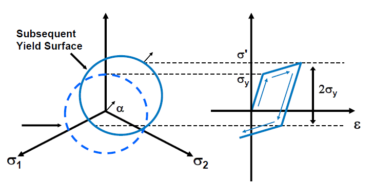
The material begins yielding at the point σy, and it is loaded into the plastic region. Loading and unloading to zero stress will not cause any additional translation of the yield surface since translation will only occur during plastic straining.
Loading into compression, produces a very different response in kinematic hardening since reverse yielding will occur at a stress of which is significantly less than or the first yield stress σ.
In order to model the Bauschinger effect, the kinematic hardening rule is used where a hardening in tension will lead to a softening in a subsequent compression.
A way to conceptualize Bauschinger effect (cyclic plasticity) behavior is to observe that the center of the yield surface moves in a direction of the plastic. The expansion of a circular yield surface corresponds to isotropic hardening and translation of its center corresponds to kinematic hardening. The isotropic hardening accords to the yield surface expansion but its center does not move. In the kinematic hardening, the center of yield surface moves but its surface does not expand.
Linear Kinematic Hardening
For linear kinematic hardening, the yield surface translates as a rigid body during plastic flow.
The elastic region is equal to twice the initial yield stress. Subsequent yield in compression is decreased by the amount that the yield stress in tension increased, so that 2σy difference between the yields is always maintained (This is known as the Bauschinger effect).
The hardening law predicts that the stress-plastic strain curve is a straight line.
There are some characteristic properties of nonlinear kinematic hardening:
- Most metals exhibit kinematic hardening behaviour for small strain cyclic loading, and kinematic hardening is generally used for small strain cyclic loading applications.
- Linear kinematic hardening is recommended for situations where the strain levels are relatively small (less than 10% true strain).
The yield criterion can be expresses as:
F = [(3/2) (s − a) : (s − a)]1/2 – σy = 0
S : Deviatoric stress
σy : Uniaxial yield stress
α : Back stress
The back stress is linearly related to plastic strain via:
Δα = [2÷3 c.Δεpl]
Nonlinear Kinematic Hardening
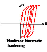
Nonlinear kinematic hardening is similar to linear kinematic hardening except for the fact that the evolution low has a nonlinear term “recall term”.
The relation can model cyclic creep, the tendency of the material to accumulate strain in the direction of the mean stress under cyclic loading. It is known as the Armstrong-Frederick hardening law.
Nonlinear kinematic hardening has got the following characteristics:
- Nonlinear kinematic hardening does not have a linear relation between hardening and plastic strain.
- Unlike linear kinematic hardening, the yield surface cannot translate forever in principal stress space.
- The constant R is added on the response.
- Nonlinear kinematic hardening is suitable for large strains and cyclic loading, as it can simulate the Bauschinger effect.
The yield criterion can be expresses as:
F = [(3/2) (s − a) : (s − a)]1/2 – R – σy ≤ 0
S : Deviatoric stress
σy : Initial yield threshold value
a : Back stress by the Armstrong-Frederick model
R : Constant yield stress
Sources:
mae.ufl.edu
wikipedia.org
auckland.ac.nz
sciencedirect.com