Explicit integration performs a key role in many analysis of linear and non-linear dynamics. The finite element method applies to spatial discretization in a system of ordinary differential equations to be solved, which is often done by the central difference method.
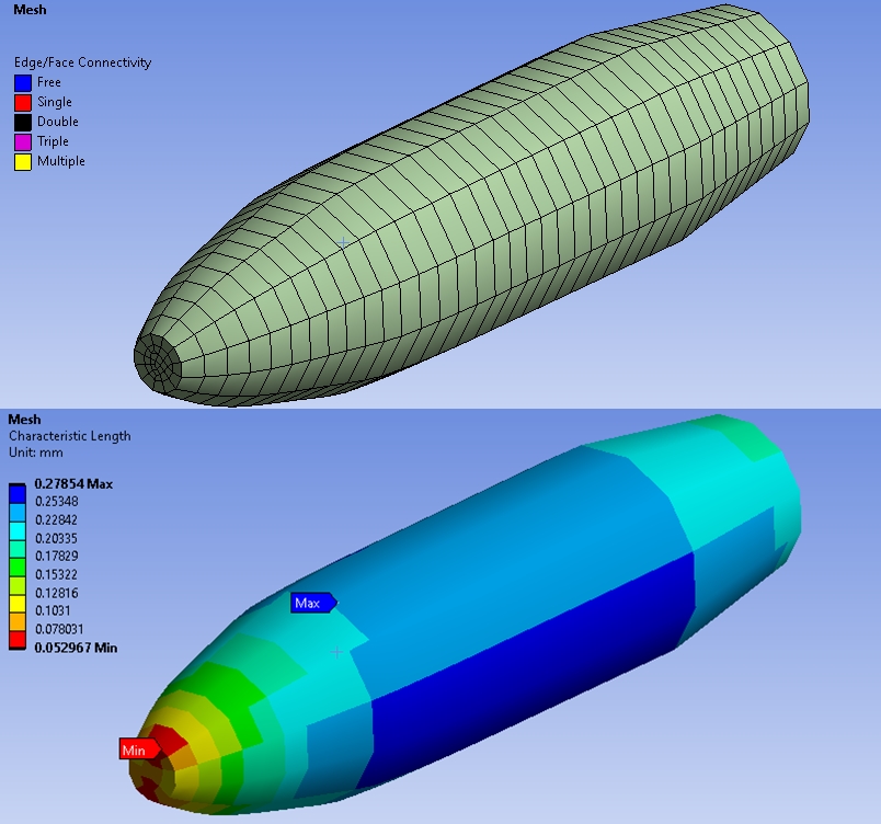
Characteristic length is an important dimension that defines the scale of a physical system. Often, such a length is used as an input to a formula in order to predict some characteristics of the system, and it is usually required by the construction of a dimensionless quantity.
In computational mechanics, a characteristic length is defined to force localization of a stress softening. The length is associated with an integration point. In 2D analysis, it is calculated by taking the square root of the area. In 3D analysis, it is calculated by taking the cubic root of the volume associated to the integration point.
A characteristic length is usually the volume of a system divided by its surface.
For more detail: Implicit vs Explicit Approach in FEM
Effects of Element Shape
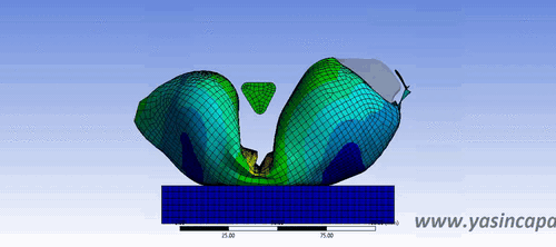
It is well-known that the critical time step is proportional to the element size (usually taken the smallest distance between any two non-adjacent edges or faces of the element), the effects of non-regular element shapes seem to have received far less attention in the literature.
Computation of the Characteristic Lengths
The computation of the stabilization parameters is a crucial issue as the effects of the stability and accuracy of the numerical solution.
The different procedures compute the stabilization parameters that are typically based on stabilized equations.
Explicit time integration methods are the most popular methods to solve the dynamic equations of fast-transient processes. Combined with lumped mass matrices, explicit algorithms require minimal CPU time and computer memory per time step, and they are very simple to implement. The time step used for time integration must be chosen smaller than critical time step for the simulation to stay stable.
Critical Time-Step
Explicit time-integration methods for FEA determines the unknowns for the next time-step in terms of quantities computed at the current or previous time-step. The explicit method requires the time-step “Δt” to supply the “C” condition in order to ensure numerical stability.
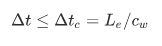
Δtc = Critical Time-Step
Lc = Characteristic Length
cw = Wave Propagation Speed
In an explicit FEA, Δt must be sufficiently small so that the wave cannot propagate across more than one element within each time-step. The critical time-step depends on material properties as well as element size and shape. For numerical stability, the critical time-step must be calculated at each time instant for each element.
The numerical time-step is determined by the smallest element in the FEM for a specified material. A well-planned uniform mesh is a general guideline to reduce the computational time (with high critical time-step) in an explicit FEA.
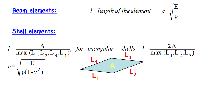
The characteristic length “l” and the wave propagation velocity “c” are dependent on element type.
E = Young’s Modulus of Elasticity
v = Poisson’s Ratio
p = Specific Mass Density
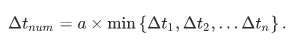
Controlling the Critical Time Step
The wave speed of the material, the nature of the higher-order eigenmodes of the finite element, and the element geometry are considered to determine the critical time step. This knowledge has been used in the literature to control, and operate the critical time step. The critical time step is set by the largest eigenvalue. Therefore, physical properties might be adjusted such that the larger eigenvalues are lowered, whereas the small eigenvalues remain unaffected.
Sources:
engmech.cz
compassis.com
dynasupport.com
sciencedirect.com